Singular Value Decomposition
Overview
Singular Value Decomposition (SVD) is one of the most fundamental matrix factorizations in linear algebra. While SVD is applicable to any matrix, EVD is only applicable to square matrices. Here, we will explore the relationship between SVD and EVD.
Mathematical Foundations
Definition
For any matrix \(A \in \mathbb{R}^{m \times n}\), SVD factorizes it as:
\[A = U \Sigma V^T\]
where: - \(U \in \mathbb{R}^{m \times m}\) — orthogonal matrix of left singular vectors (columns are eigenvectors of \(AA^T\)) - \(\Sigma \in \mathbb{R}^{m \times n}\) — rectangular diagonal matrix of singular values \(\sigma_1 \geq \sigma_2 \geq \cdots \geq \sigma_r \geq 0\) - \(V \in \mathbb{R}^{n \times n}\) — orthogonal matrix of right singular vectors (columns are eigenvectors of \(A^T A\))
The orthogonality conditions are:
\[U^T U = I_m \qquad V^T V = I_n\]
The Singular Values
The singular values are defined as the square roots of the eigenvalues of \(A^T A\) (or equivalently \(A A^T\)):
\[\sigma_i = \sqrt{\lambda_i(A^T A)}, \quad i = 1, \dots, r = \text{rank}(A)\]
The diagonal matrix \(\Sigma\) looks like:
\[\Sigma = \begin{pmatrix} \sigma_1 & & & \\ & \sigma_2 & & \\ & & \ddots & \\ & & & \sigma_r \\ & & & & \ddots \end{pmatrix}\]
with zeros outside the main diagonal.
Deriving the Singular Vectors
Right singular vectors \(v_i\) (columns of \(V\)) satisfy:
\[A^T A \, v_i = \sigma_i^2 \, v_i\]
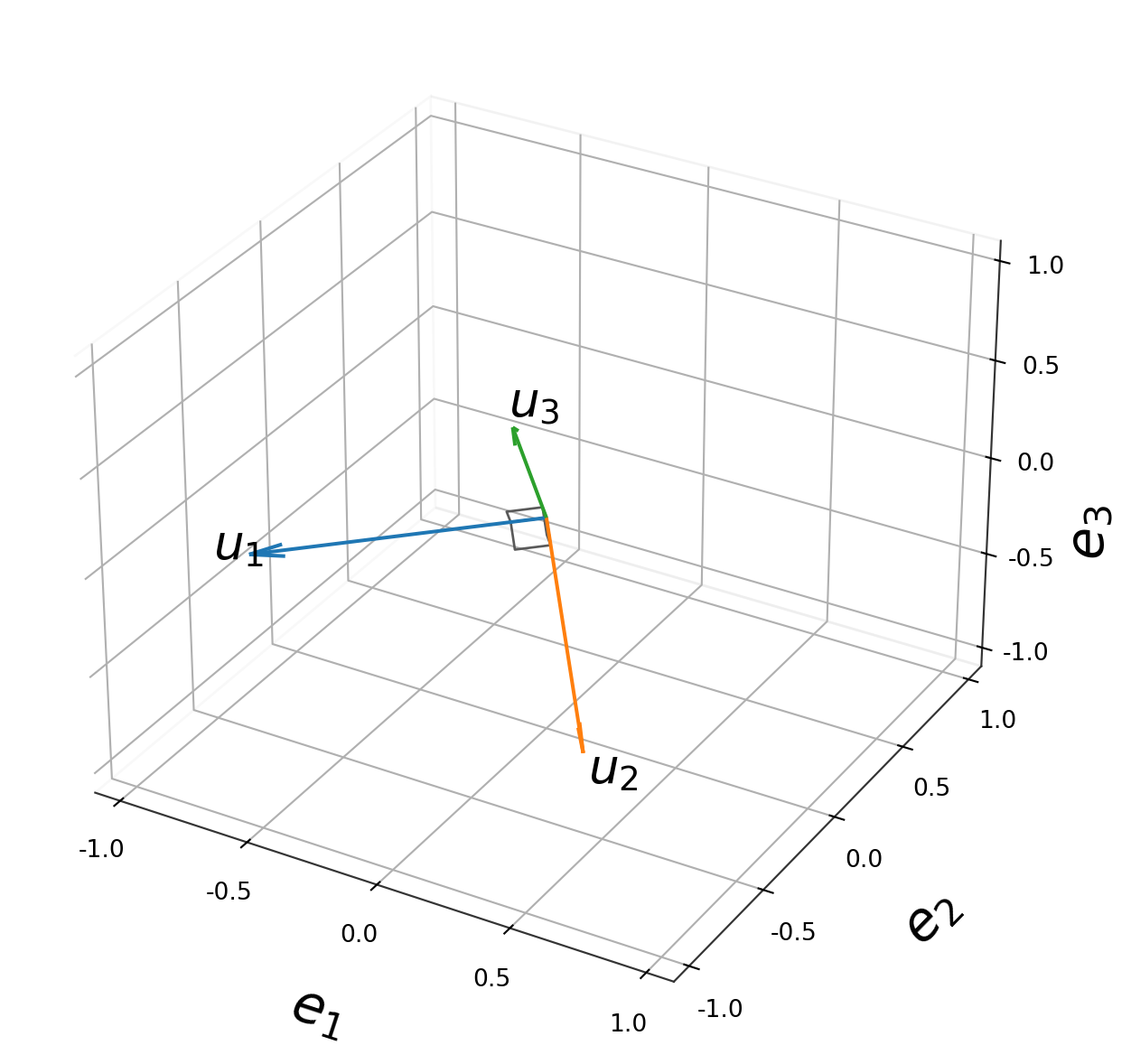
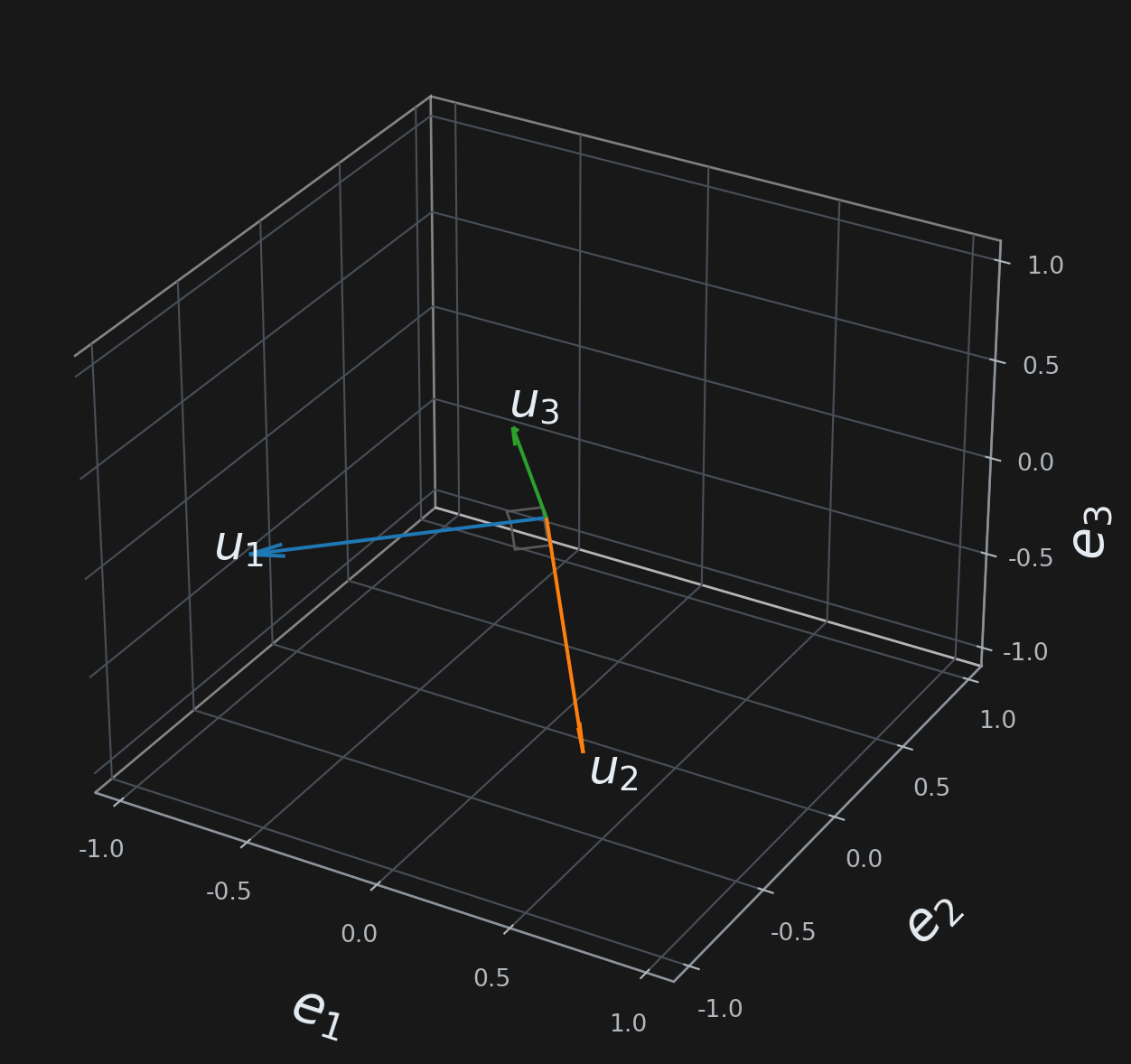
Left singular vectors \(u_i\) (columns of \(U\)) are then obtained via:
\[u_i = \frac{1}{\sigma_i} A v_i\]
This satisfies the core SVD relationship:
\[A v_i = \sigma_i u_i \qquad \Longleftrightarrow \qquad A V = U \Sigma\]
Compact (Thin) SVD
For rank-\(r\) matrix \(A\), only \(r\) singular values are non-zero. The thin SVD keeps only the meaningful part:
\[A = U_r \Sigma_r V_r^T\]
where \(U_r \in \mathbb{R}^{m \times r}\), \(\Sigma_r \in \mathbb{R}^{r \times r}\), \(V_r \in \mathbb{R}^{n \times r}\).
Outer Product (Sum) Form
SVD can be written as a sum of rank-1 matrices:
\[A = \sum_{i=1}^{r} \sigma_i \, u_i v_i^T\]
This is extremely useful — you can truncate the sum to get the best rank-\(k\) approximation (Eckart–Young theorem):
\[A_k = \sum_{i=1}^{k} \sigma_i \, u_i v_i^T = \underset{\text{rank}(B)=k}{\arg\min} \| A - B \|_F\]
SVD vs. EVD — Key Differences
| Property | SVD | EVD |
|---|---|---|
| Applicable to | Any \(m \times n\) matrix | Square \(n \times n\) matrices only |
| Factorization | \(A = U\Sigma V^T\) | \(A = Q\Lambda Q^{-1}\) |
| Two vector spaces | Left (\(U\)) and right (\(V\)) are different | Same vector space for input and output |
| Values on diagonal | \(\sigma_i \geq 0\) always real, non-negative | \(\lambda_i \in \mathbb{C}\) can be complex |
| Factor matrices | \(U, V\) always orthogonal | \(Q\) orthogonal only if \(A\) is symmetric |
| Uniqueness | Always exists | May not exist (defective matrices) |
| Geometry | Rotation → stretch → rotation | Stretch along eigenvectors |
The Deep Connection
For a symmetric positive semidefinite matrix \(A = A^T \geq 0\), SVD and EVD coincide:
\[A = Q\Lambda Q^T = U\Sigma V^T \quad \Rightarrow \quad U = V = Q, \quad \Sigma = \Lambda\]
For a general square matrix \(A\), SVD works on \(A^T A\) and \(AA^T\):
\[A^T A = V \Sigma^T \Sigma V^T \quad \text{(eigendecomposition of } A^T A\text{)}\] \[A A^T = U \Sigma \Sigma^T U^T \quad \text{(eigendecomposition of } A A^T\text{)}\]
So singular values of \(A\) are the square roots of eigenvalues of \(A^T A\):
\[\sigma_i(A) = \sqrt{\lambda_i(A^T A)}\]